I recently took up a job that requires me to be involved in structural analysis once again, which naturally means I need to refresh my fundamentals in mathematics and strength of materials (the basis of structural and mechanical engineering). To benefit some of my readers, I’ve decided to share this learning process with my audience.
The feedback I've received thus far has been positive, and I’m pleasantly surprised at how many readers of this blog, despite working in fields that don't directly demand mathematical knowledge, still maintain an interest in the subject.
With time, I will publish most of my notes on this blog. Converting my notes into the language in which they were originally written (whether Afrikaans, German, or French) is a challenging task. I apologize to my audience who understands multiple languages, as you may receive duplicate copies via email. As you will notice, there are subtle differences in how mathematics is communicated in each language. These differences are not related to the concepts themselves but rather to slight variations in teaching methods across different countries. Mathematics is a universal language.
I am doing this for several reasons. Firstly, I believe that revisiting the basics of any subject is important. We often think we have a solid grasp of fundamental concepts, only to rediscover deeper insights along the way. Secondly, I find that if I can communicate complex ideas to a lay audience, it becomes easier to communicate them to engineers and scientists (who often suffer from 'the curse of knowledge'—being so knowledgeable that we forget what we've learned and others haven't). Lastly, and most importantly, my wife is a mathematician, and if our daughter is going to school one day, we may be better prepared for what she might encounter, because we too forgot the basics.
The best way to show how going back to the basics reveals deeper insights is by revisiting the Pythagorean theorem. Although the Greeks like Pythagoras were the first to formalise it, we shouldn’t forget that the Persians, Mayans, and Babylonians also had knowledge of its application.
The Pythagorean theorem is arguably the most well-known theorem in mathematics and is one of the first lessons that school children encounter in geometry, trigonometry or algebra. I still recall how our mathematics teacher made us mémorise the following equation:
c² = a² + b²
with
c the hypotenuse of the right handed triangle
a the adjacent edge of the right handed triangle
b the opposite edge of the right handed-triangle
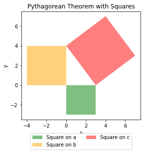
It is often presented with on a graph such as the following.
More formally, the theorem states that in a right-angled triangle, the square of the length of the hypotenuse is equal to the sum of the squares of the lengths of the other two sides.
One can obviously measure the squares and conclude that the theorem holds, but for purists in mathematics, this is not sufficient, as the proof must be “rigorous and demonstrated to hold under all conditions”.
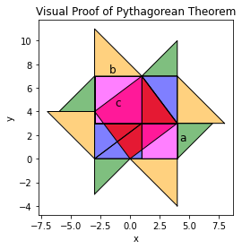
There are several ways to proof that the relationship c² = a² + b² holds, but one of my favorites is to slice the squares on b and c into two equal halves, forming triangles of equal size.
The trick is to slide the triangles around the red square, creating a copy of each square helps.
The blue triangles that form are now of interest.
They too can be slid over, forming new two blue rectangles. For clarity, I made the red square in the center completely transparent.
The pink squares that form share the sides of the green and yellow triangles, and therefore they should have areas of a² and b², respectively. Since the area of the larger rectangle (with length a+b) remains unchanged, it follows that the combined area of the pink squares must be equal to the red square, because shuffling the blue squares around didn’t change the dimensions of the rectangle.
Thus, it must hold that c²=a²+b², which is the formula of the Pythagorean theorem.
For completeness sake, the square is added in the following figure.
Now by looking a bit more closely at the graph, another interesting fact is revealed: the formula for the expansion of squares!
Notice that when the inner square is removed, area of the larger rectangle (the sum of the pink squares and blue triangles) is equal to.
(a+b)²=a²+b²+4(0.5ab) = a²+b²+2ab
This is a geometric demonstration of the expansion of squares and the term 2ab is actually the area of the 4 blue triangles (each being equal to 0.5ab).
The proof of the Pythagorean Theorem therefore holds an additional truth, which is a geometric demonstration of the expansion of squares.
The python code is below for those who are interested in playing around with it.
"""
By Hügo KRÜGER
demonstration of the proof of the Pythagorean Theorem,
The proof uses the triangles and squares of the adjacent
and opposite edge of the right triangle.
For more information go to https://hkrugertjie.substack.com/


"""

import matplotlib.pyplot as plt
import numpy as np

# Example values for a and b (legs of the right triangle)
a = 3
b = 4
c = np.sqrt(a**2 + b**2)  # Hypotenuse calculated by Pythagoras

# Coordinates for the square (on the hypotenuse side)
square_a_coords = [[0, a, a, 0], [0, 0, a, a]]  # Square on side a
square_b_coords = [[0, b, b, 0], [0, 0, b, b]]  # Square on side b
square_c_coords = [[0, c, c, 0], [0, 0, c, c]]  # Square on hypotenuse

# Translate squares
square_a_translation = (-a+b, 0)
square_b_translation = (-a, a)

# Coordinates for 12 triangles
triangle_coords = [
    ([0, a, a], [-a, -a, 0]),  # Triangle 1
    ([0, a, 0], [-a, 0, 0]),    # Triangle 2
    ([0, 0, -b], [0, b, b]),    # Triangle 3
    ([0, -b, -b], [0, b, 0]),   # Triangle 4
    ([0, a, a], [-a, -a, 0]),  # Triangle 5 (duplicate)
    ([0, a, 0], [-a, 0, 0]),    # Triangle 6 (duplicate)
    ([0, 0, -b], [0, b, b]),    # Triangle 7 (duplicate)
    ([0, -b, -b], [0, b, 0]),   # Triangle 8 (duplicate)
    ([0, b, b], [0, 0, a]),   # Triangle 9 (inner)
    ([b, b, b-a], [a, a+b, a+b]),  # Triangle 10 (inner)
    ([b-a, -a, -a], [a+b, a+b, b]),  # Triangle 11 (inner)
    ([0, -a, -a], [0, b, 0])      # Triangle 12 (inner)
]

# Rotation angles and translations (no rotation for any triangles)
angles = [0] * 12
translations = [
    (b-a, 2*a+b),  # No translation for the first triangle
    (b, a),  # Move the second triangle to the right of the first
    (b, -b),  # Move the third triangle upwards
    (2*b, a),  # Move the fourth triangle to the top right corner
    (-a*2, b+a),  # Move the fifth triangle
    (-a, 0),  # Move the sixth triangle
    (-a, 0),  # Move the seventh triangle
    (b-a, a+b),  # Move the eighth triangle
    (-a, 0),  # Move the ninth triangle
    (0, 0), # Move the tenth triangle
    (0, -b), # Move the eleventh triangle
    (b, a)   # Move the twelfth triangle
]
triangle_colors = ['green', 'green', 'orange', 'orange', 'green', 'green', 'orange', 'orange', 'blue', 'blue', 'blue', 'blue']

# Create the plot
fig, ax = plt.subplots()

# Plot triangles with rotation, translation, and color
for (x, y), angle, translation, color in zip(triangle_coords, angles, translations, triangle_colors):
    x_rot, y_rot = np.dot([[np.cos(angle), -np.sin(angle)], [np.sin(angle), np.cos(angle)]], [x, y])
    x_rot += translation[0]
    y_rot += translation[1]
    ax.fill(x_rot, y_rot, color, alpha=0.5)
    ax.plot(np.append(x_rot, x_rot[0]), np.append(y_rot, y_rot[0]), color='black', linewidth=1)

# Function to apply rotation and translation to square coordinates
def rotate_and_translate_square(coords, angle, translation):
    rotation_matrix = np.array([[np.cos(angle), -np.sin(angle)], [np.sin(angle), np.cos(angle)]])
    x_rot, y_rot = np.dot(rotation_matrix, np.array([coords[0], coords[1]]))
    return x_rot + translation[0], y_rot + translation[1]

# Plot squares with original rotation logic
square_rot_angle = np.arctan(a / b)

# Plot the square on the hypotenuse
square_rot_x, square_rot_y = rotate_and_translate_square(square_c_coords, square_rot_angle, (0, 0))
ax.fill(square_rot_x, square_rot_y, 'red', alpha=0.8)
ax.plot(np.append(square_rot_x, square_rot_x[0]), np.append(square_rot_y, square_rot_y[0]), color='black', linewidth=1)

# Plot the square on side a
square_a_x, square_a_y = rotate_and_translate_square(square_a_coords, 0, square_a_translation)
ax.fill(square_a_x, square_a_y, 'magenta', alpha=0.5)
ax.plot(np.append(square_a_x, square_a_x[0]), np.append(square_a_y, square_a_y[0]), color='black', linewidth=1)

# Plot the square on side b
square_b_x, square_b_y = rotate_and_translate_square(square_b_coords, 0, square_b_translation)
ax.fill(square_b_x, square_b_y, 'magenta', alpha=0.5)
ax.plot(np.append(square_b_x, square_b_x[0]), np.append(square_b_y, square_b_y[0]), color='black', linewidth=1)

# Annotate sides a, b, and c
ax.text(-a/2, a+b+0.3, 'a', fontsize=12, color='black', ha='center')
ax.text(b+0.5, a/2, 'b', fontsize=12, color='black', ha='center')
ax.text(-1, b+a/2-1, 'c', fontsize=12, color='black', ha='center')

## Set plot properties for equal scaling and unit length
ax.set_aspect('equal', 'box')
# ax.set_xlim(-b, 2*b)  # Adjust x-axis limit based on the largest side
# ax.set_ylim(-4*b, max(-2*b, 1))  # Adjust y-axis limit based on the largest side
ax.set_xlabel('x')
ax.set_ylabel('y')
ax.set_title('Visual Proof of Pythagorean Theorem')


# Show the plot
plt.show()


